Introduction

In the dynamic world of business, decision-making is crucial. From logistics management to staffing optimization, businesses rely on data-driven insights to stay competitive. This blog explores four real-world business problems and how data analytics can provide actionable solutions.

Case: 1

Swift Shipping: Decision Analysis Regarding Postal Strike Threat

The Problem

Swift Shipping, a Glasgow-based clothing retailer, faces a potential postal strike that could disrupt next-day delivery services. The Operations Manager must decide whether to:

• Ship as usual and risk costly delays if a strike occurs.

• Preemptively postpone shipments to mitigate risk.

• Invest in acquiring strike probability data to make an informed decision.

Business to Statistical Questions

• What is the probability threshold at which postponing shipments minimizes expected costs?

• How does acquiring additional data impact decision-making regarding strike probability?

• What is the expected value of additional information (EVI) for different strike probabilities?

Statistical Analysis Approch

• Construct a decision tree to estimate the probability cutoff for shipping decisions.

• Use Bayesian analysis to quantify the impact of purchased strike data.

• Calculate the EVI for various probability ranges and recommend optimal strategies.

Analysis

This report analyses the optimal strategy for Swift Shipping regarding a potential postal strike before the busy season. Considered the costs of shipping normally, postponing shipments, and acquiring strike likelihood data.

Key Findings:

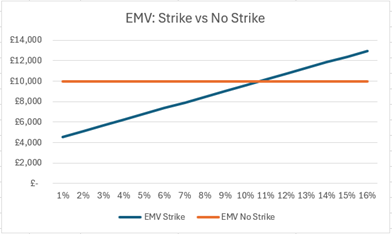
• Shipping is normally preferred when the strike probability is below 11%.

• Purchasing strike likelihood data (costing £1,000) provides significant benefit at a strike probability of 15% (p = 0.15).

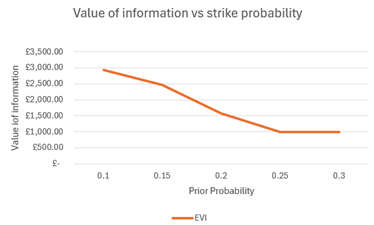
• The expected value of information (EVI) for purchasing strike data is higher if the probability of a strike is below 25%. Above 25%, the value of information is £1,000, indicating that the cost outweighs the benefit.

Recommendation:

Based on the analysis, Swift Shipping should proceed with regular shipping via Scottish couriers before the busy season if the estimated strike probability remains below 11%. To minimise the costs, they should buy the strike likelihood data. If the strike probability is below 25%, Swift Shipping can invest up to £3,000 in buying the data; if it is above 25%, they are not advised to spend more than £1,000. This approach minimises expected costs compared to postponing shipments.

Quantitative Support:

• Shipping usually costs £4,000 if no strike occurs, which is lower than the £10,000 cost of postponing regardless of the strike.

• At p = 0.15, the expected cost with strike data is approximately £8,540, whereas shipping typically has an expected cost of around £10,000.

Limitations, Risks, and Mitigation Strategies:

• The analysis assumes accurate strike probability and estimations of cost figures, but unexpected changes in these factors could influence the optimal strategy.

• There’s inherent uncertainty in strike predictions. Even with perfect data, strikes could still occur unexpectedly.

• Mitigation strategies for potential delays due to strikes include:

  • Identifying alternative couriers outside of Scotland as a backup.

  • Communicating transparently with customers about potential delays.

  • Exploring options for expedited shipping methods if necessary.

Conclusion:

By proceeding with regular shipping unless the strike probability significantly increases, Swift Shipping can minimise expected costs and maintain customer expectations for next-day delivery. The Operations Manager should continuously monitor the strike situation and adjust the strategy if the probability of a strike rises above the critical threshold (around 11%). To improve the judgement of strike, buying strike likelihood data is beneficial. Implementing the suggested mitigation strategies can further reduce risks associated with potential delays.

Case: 2

Optimizing Staffing at Newcastle University’s Credit Union

The Challenge

Newcastle University’s credit union faces unpredictable customer footfall, leading to long queues on some days and idle staff on others. Manager Michael Kaluuya needs a forecasting model to optimize staffing.

Business to Statistical Questions

• How can historical data be used to predict daily customer arrivals?

• What independent variables significantly impact footfall predictions?

• What statistical model best balances accuracy and interpretability for staffing decisions?

Statistical Analysis Approch

• Build a multiple linear regression model using relevant variables (day, payday effects, etc.).

• Identify statistically significant predictors using p-values and confidence intervals.

• Evaluate model fit using R-Squared and Adjusted R-Squared metrics.

Analysis

This report details the development of a powerful new tool to predict how many customers will visit your credit union branch at Newcastle University each day. This model will significantly improve staff scheduling, reduce wait times, and enhance customer service.

Model Methodology:

The final model employs a multiple linear regression approach. This model predicts the daily number of customer arrivals (“Arrivals”). To predict the accurate number of daily customer arrivals, this model investigates these factors:

• Basic factors (Independent Variables):
  • What day of the week it is (e.g., Monday, Tuesday)
  • What day of the month it is (e.g., 1st, 2nd)
  • Whether there’s a staff or faculty payday
  • Whether it’s before or after a holiday
• Advanced factors (Derived independent variables):
  • Lag of 1 (Arrival) – Lag of 20 (Arrival):

    • It captures the last 20 days (one work month) of daily customer arrivals.

    • It Captures the short-term and potentially cyclical patterns.

Model Performance:

• Multiple R: 0.9168
  • It shows a strong positive relationship between the above basic and advanced factors (All independent variables) and daily customer arrivals.
• R-Squared: 0.8405
  • this model performs well in explaining 84.05% of the variation in daily customer arrivals.
• Adjusted R-Squared: 0.8325
  • Based on the complexity of the model, it indicates all the basic and advanced factors (All independent variables) fit perfectly.
• Standard Error of Estimate: 138.77
  • on average, the model’s prediction will differ from the number of daily customer arrivals by 139 customers.

Model Evaluation:

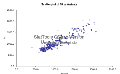
• Linearity: Fitted values vs actual Y value plot shows a positive linear correlation between points. This suggests that the model’s predictions (fitted values) increase as the actual arrival values (Y values) increase. This is a good sign because it suggests that the linear regression model captures the underlying trend in the data.

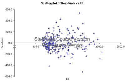
• Homoscedasticity: Residuals vs fit plot shows random points scattered around zero, indicating no apparent pattern. This suggests that all the daily customer arrival data points are given the same attention for prediction; that’s why there is no pattern upholding the assumption of homoscedasticity.

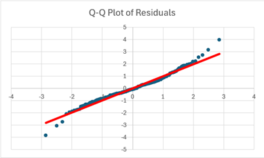
• Normality of Errors: The residuals’ Q-Q plot resembles a 45-degree line with minor deviations at the beginning and end. This model can capture general trends. Still, it won’t be able to predict correctly for unexpected fluctuations, and more data is needed to capture these non-linear relationships.

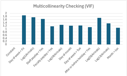
• Multicollinearity: The selection of only important variables reduced the complexity of the model, and the Variance Inflation Factor (VIF) for all independent variables is below 2, indicating a low risk of multicollinearity.

Linear regression Equation:

The linear regression Equation for the model shows that Fridays have a coefficient of +425.96, meaning it is expected that there will be 426 more customer arrivals on Fridays compared to a reference day, like Monday, which likely has a coefficient close to zero. Tuesdays have a coefficient of -74.37, indicating typically fewer arrivals on Tuesdays. Both staff and faculty paydays have positive coefficients (around +303 each). This means there is an expectation of an increase in arrivals on these days compared to non-payday periods. Days before or after a holiday have a coefficient of +160.54, suggesting more customer activity around holidays. Yesterday’s arrivals have the strongest influence, with a coefficient of 0.3377. This translates to an estimated increase of 0.34 arrivals today for every additional arrival yesterday. The impact weakens as looked further back, with arrivals from 19 days ago and arrivals from 20 days ago having coefficients of around 0.11 and 0.12, respectively.

Overall Assumption Evaluation:

The model’s assumptions are met reasonably well based on the analysis of the fitted values vs actual Y value plot, residuals vs fit plot, multicollinearity of independent variables, and Q-Q plot. However, it’s essential to acknowledge the minor deviations from normality observed in the Q-Q plot, which shows the model cannot give 100% correct answers. However, Future data can help refine its ability to capture these potential non-linearities. Overall, this model has high accuracy in predicting the correct number of arrivals with some errors.

Exploratory Data Analysis and Insights

Data analysis reveals several vital patterns and trends influencing daily customer arrivals at the credit union branch, supporting model assumptions. More Graphs are presented in Appendix A.

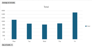
Figure: Fridays see significantly higher customer traffic than other weekdays

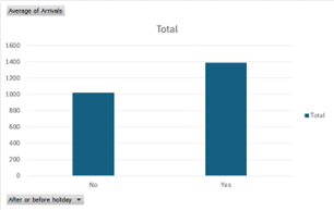
Figure: More Arrivals if the day is around a holiday.

Strengths and Limitations

• Strengths:

  • The model incorporates factors influencing customer arrivals, leading to more accurate predictions.

  • The previous 1 week of arrivals helps in taking account of short-term seasonality and identifying trends.

• Limitations:

  • The model may not capture unexpected events (like strikes) causing fluctuation in customer arrivals.

  • Over time, customer behaviour and branch operations might change. This “data drift” can gradually make the model’s predictions less accurate.

Recommendations

• Regularly monitor model performance and retrain it periodically with new data to maintain accuracy.

• Consider incorporating additional factors like weather data or special events if significant correlations are suspected.

• Explore alternative modelling techniques (e.g., time series forecasting) if the assumptions of linear regression are violated.

Case: 3

Production Optimization at Zahret Company

The Problem

Zahret Company produces two products with limited labor hours across three departments. Management seeks to maximize profit while balancing labor constraints.

Business to Statistical Questions

• How can production be optimized within given labor constraints to maximize profit?

• What is the shadow price of labor in different departments?

• How does overtime availability affect the optimal production levels?

Statistical Analysis Approch

• Formulate and solve a linear programming model to determine optimal production quantities.

• Analyze shadow prices to determine the marginal benefit of additional labor.

• Introduce overtime variables and re-optimize production plans accordingly.

• Inventory Management Simulation for Paxon Pharma

Analysis

This report summarises the analysis to optimise production levels for Products 1 and 2 at Zahret Company. Utilising a linear programming model to identify the most profitable production plan while considering labour constraints.

Initial Model

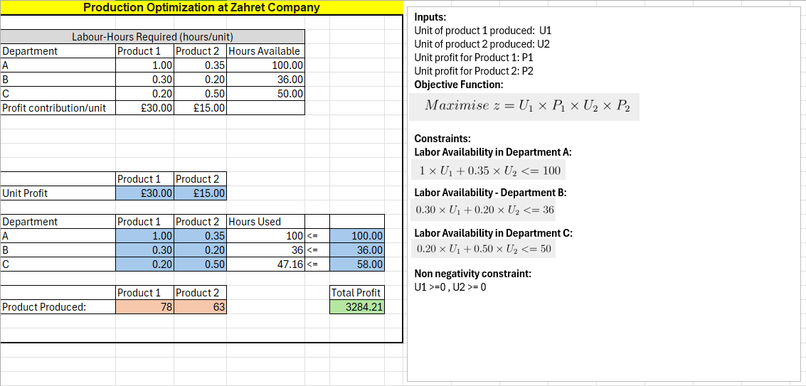
• The initial model assumed fixed labour availability. The optimal solution suggests producing 78 units of Product 1 and 63 units of Product 2, resulting in a total profit contribution of £3,284.21.

Overtime Considerations

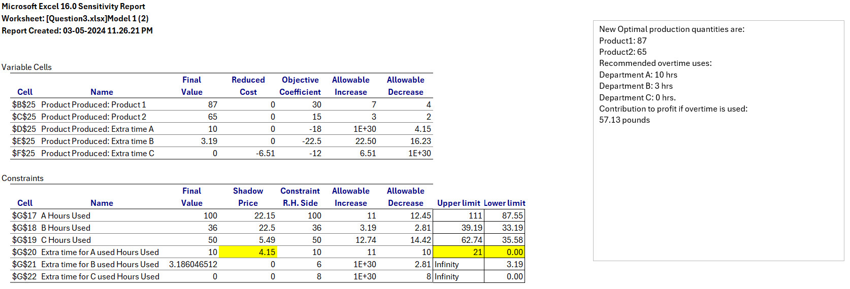
• When incorporating potential overtime costs, the analysis considered the “shadow price” for each department. This represents the additional profit per unit of labour available in each department. Departments A and B had positive shadow prices, indicating that overtime in those departments could be beneficial.

• Based on this analysis, exploring overtime options in Departments A and B is recommended. The model suggests a maximum overtime cost of £15.79 per hour in Department A and £47.37 per hour in Department B.

Model with Overtime Implementation

• The model incorporates available overtime hours (10 hours in A, 6 hours in B, and 8 hours in C) and their associated costs (£18, £22.50, and £12 per hour, respectively).

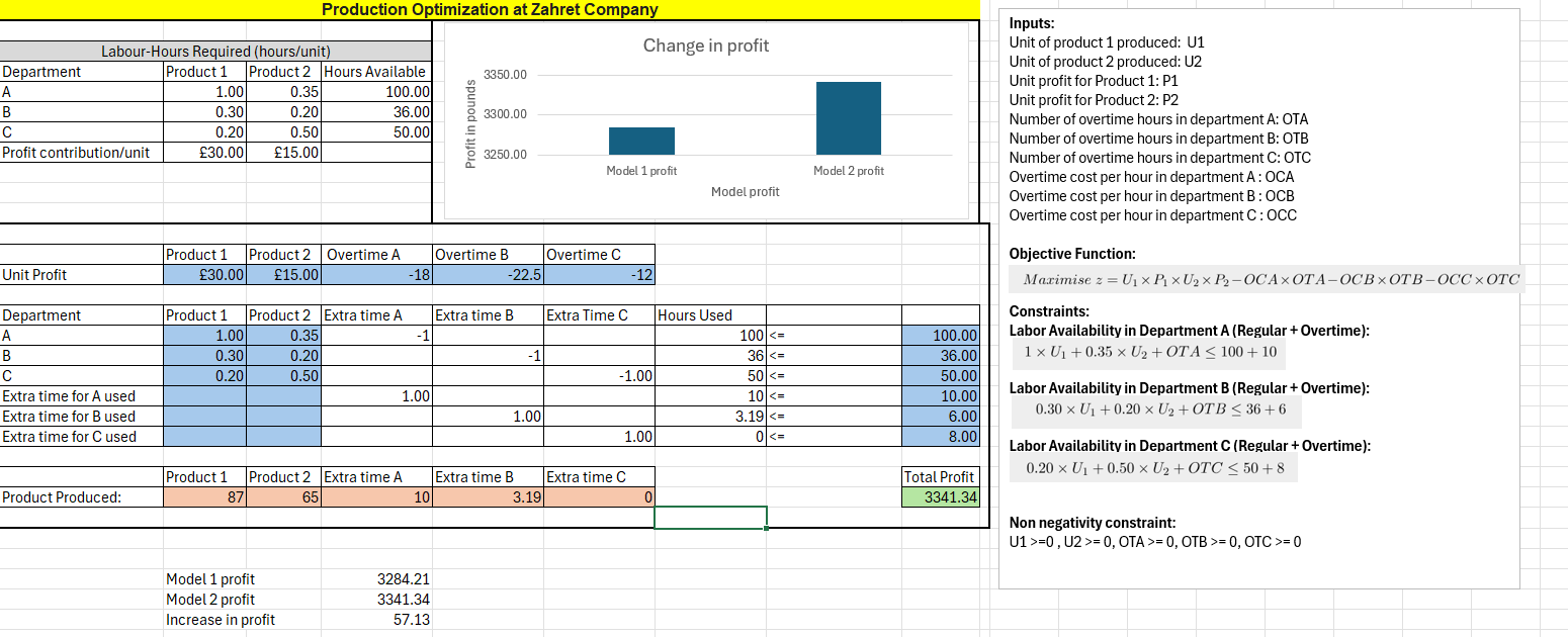
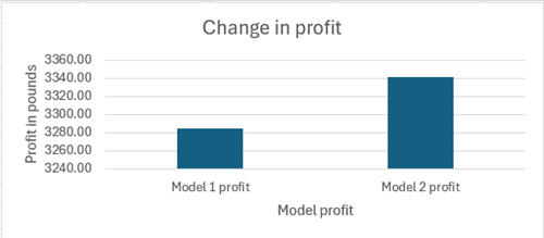
Figure: showing a profit for the initial model (model 1) and the new model with overtime considerations (model 2).

• The revised model recommends producing 87 units of Product 1 and 65 units of Product 2. This revised plan leads to a total profit contribution of £3,341.34, representing an increase of £57.13 due to the efficient use of overtime.

• The optimal overtime usage is 10 hours in Department A and 3 hours in Department B. While overtime is available in Department C, the model suggests it’s not economical at this cost.

Additional insight:

Even though 8 hours of overtime are available in Department C, reallocating them to Department A is more profitable. Since the shadow price is £4.15 in Department A and the allowed increase is 11 more hours with the same optimal solution, moving 8 hours from Department C to Department A would increase profit by around £33.

Recommendations

• Producing 87 units of Product 1 and 65 units of Product 2.

• Utilizing 10 hours of overtime in Department A and 3 hours in Department B.

Case: 4

Inventory cost management for Paxon Pharma manufactures

The Problem

Paxon Pharma manufactures amoxicillin but faces fluctuating inventory costs. Management seeks an optimal production strategy to minimize costs while avoiding lost sales.

Business to Statistical Questions

• What inventory threshold minimizes total holding and production costs?

• How does varying the upper threshold (U) impact long-term cost efficiency?

• Can a simulation-based approach provide confidence intervals for optimal policies?

Statistical Analysis Approch

• Develop a Monte Carlo simulation model to test different inventory policies.

• Run multiple iterations to estimate mean and standard deviation of costs.

• Construct confidence intervals to determine the most cost-effective production threshold.

Analysis

This report analyses a production planning policy for Paxon Pharma’s amoxicillin inventory in the UK. The simulation model suggests a clear optimal value for the upper inventory threshold (U) that minimises total cost. Limitations of the current approach and recommendations for further investigation into alternative policies are also explored.

Inventory Analysis

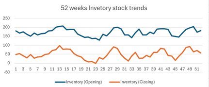
A 52-week simulation model is built in Excel to evaluate a policy with three production levels triggered by inventory levels. The above chart represents the 52 weeks of inventory (opening and closing) stock trends. Then, 500 iterations were performed, varying the upper threshold (U) from 30 to 80 units while keeping the lower threshold (L) fixed at 30.

Findings

• Optimal Upper Threshold (U): The average 52-week cost across simulations consistently decreases as U increases until 54 units and then increases, reaching a minimum of around U = 54 units, with an average weekly cost of £ 5,541.35. The average cost will be around £ 5,811.35 for 95% of the time, with a chance of deviation of £ 193.38. This indicates that holding a slightly lower inventory level up to this point reduces overall costs compared to frequent production changes.

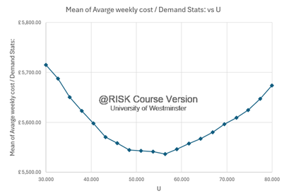
• Cost vs Upper Threshold (U): The graph depicts a downward trend in average cost as U increases until a point when it starts increasing. The optimal value of U is when the average cost in the graph is at the lowest point.

Recommendations

Based on the simulation results, setting the lower inventory threshold (U) to approximately 54 units is recommended. This strategy balances minimising frequent production adjustments with maintaining sufficient inventory to avoid lost sales.

Limitations and Further Investigation

• The current policy is a simple three-level approach. More sophisticated inventory management models could be explored.

• The simulation only considers a fixed weekly demand with a standard deviation. Optimising weekly production rates or forecasting techniques could improve the Production policy.

Conclusion

This simulation analysis provides valuable insights for Paxon Pharma’s amoxicillin inventory management. While a clear optimal upper threshold is identified, further investigation into more advanced inventory control models and incorporating optimisation of weekly production rates is recommended to optimise inventory costs in the long run.

Appendix :

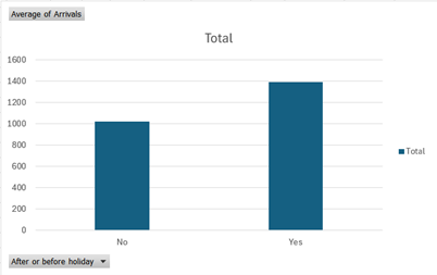
On Average, more customers visit the bank after or before the holiday.

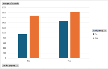
More arrivals if there is a faculty or staff payday and more footfall if there is a faculty payday.

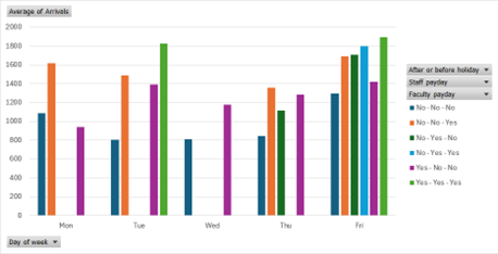
There will be more customer arrivals if there is a faculty payday, staff payday, or holiday after or before the day.

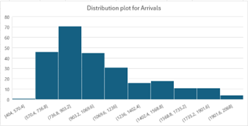
The distribution curve shows it is a positively skewed distribution. It shows that the customer’s arrival is different throughout the year. Generally, it stays on the lower side, but a few times, there are more customer arrivals.

Final Thoughts

From logistics and staffing to production and inventory management, data analytics is an invaluable tool for business success. By converting business problems into statistical questions and leveraging models, businesses can make informed decisions that drive efficiency and profitability.

Disclaimer

This report was originally submitted as part of the coursework requirements for the Master of Science in Data Science and Analytics at the University of Westminster. The content reflects the author's academic research and findings at the time of submission.

While efforts have been made to ensure accuracy, the report may not be free from errors or may not reflect the most current developments in the field. The views and conclusions expressed are those of the author and do not necessarily represent those of the University of Westminster or any affiliated institution.

This document is provided for informational and educational purposes only. It should not be used as a substitute for professional advice or as an official representation of industry standards. The author and the University of Westminster disclaim any liability for any direct or indirect consequences resulting from the use of this material.

For any inquiries or permissions regarding the reproduction of this work, please contact the author.